|
Characteristic Curves
It is possible to obtain an accurate measure of the potential performance of any valve by examining the characteristic curves for it which are published by the valve manufacturer. A characteristic curve for a valve is a graph which shows the relationship between two electrical quantities interrelated by way of the valve itself. In many instances, characteristic curves for a valve may be drawn by the student or experimenter, since the only equipment required consists of several simple meters and sources of supply.
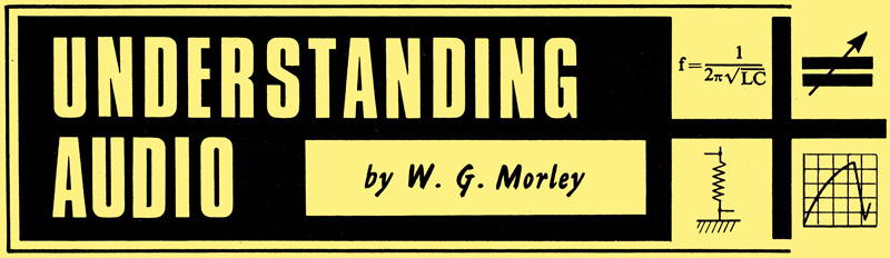
A circuit suitable for plotting the IaVa curve of a diode.
In the above diagram we set up a circuit for obtaining the anode current-anode voltage characteristic curve of a diode. The equipment employed comprises the diode itself, whose heater is supplied by a battery or other source of EMF, a current-reading meter in series with the anode, and a variable source of positive voltage (relative to cathode). This last voltage is very conveniently provided by a potentiometer connected across a second battery, and a voltmeter tells us the potential between the slider of the potentiometer and the cathode. We plot the anode current-anode voltage graph by adjusting the potentiometer and noting the anode currents which flow at the voltages indicated by the voltmeter. It is assumed that the current meter is a low-resistance instrument which drops negligible voltage, whereupon the voltage indicated by the voltmeter is the anode voltage itself.
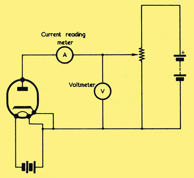
A typical IaVa curve, as would be given with the circuit in the first diagram. Anode voltage is with respect to cathode. The curve is representative of a small diode as used for HT rectification.
A typical result of such an exercise is the anode current-anode voltage characteristic curve shown above. As we would expect, this shows zero current at zero anode voltage, the current increasing as the anode voltage increases. (As we shall see later in this article a small current does in fact flow at zero anode voltage; but this does not affect the topic under immediate discussion).
However, the curve is not a straight line, as would be given if the diode were replaced by a resistor, but shows marked curvature, particularly at the ends. The curvature in the first part, from the zero point up to about point X, is due to a limitation in anode current imposed by the space charge in the diode.
The reason for current limitation due to the space charge may be understood if we consider two opposing effects. The first of these is that the space charge, consisting of a cloud of electrons around the cathode, repels the further electrons which are emitted from that cathode. The second effect is that the positive anode causes some of the electrons in the space charge to leave it and travel to the anode, and these lost electrons have to be made good by the acquisition of further electrons from the cathode. Up to about point X on the curve the second effect is of a lower magnitude than the first with the overall result that the space charge achieves a partial limitation of anode current. Put another way, it can be said that the positive anode partially, but not wholly, neutralises the repulsive effect of the space charge.
As anode voltage increases so does the second effect just referred to, and the current limitation imposed by the space charge reduces. This process continues until, at about point X, the quantity of electrons leaving the space charge is very nearly the same as the quantity emitted by the cathode, whereupon the space charge virtually disappears and very nearly all electrons leaving the cathode travel straight to the anode.
Point X is usually referred to as the saturation point and it marks the start of the condition where almost all the electrons emitted by the cathode travel towards the anode. As anode voltage increases after the saturation point the curve flattens off, because the anode is now drawing from the cathode very nearly all the electrons that it can emit. This condition is known as saturation and the diode may be referred to as being saturated.
To sum up, the curve demonstrates that anode current is limited either by the space charge or by saturation. Up to about point X the limiting factor is the space charge whilst, after point X, the limiting factor is saturation.
It might at first be thought that the curve should become almost completely flat after the saturation point has been reached because, since all (or very nearly all) the total emission of the cathode is travelling to the anode, there should then be no further significant increase in anode current. In practice, however, the flattening of the curve is not as marked as such a consideration would lead one to believe, the reason for this being that the surface of the cathode cannot be made perfectly smooth. There must always be small microscopic pockets in the cathode surface, the insides of which become hotter than the outer cathode surface and which, therefore, emit a greater proportion of electrons. Very small space charges appear immediately outside these pockets and they can only be neutralised by higher anode voltages. Thus, there is still a small increase in anode current with increase in anode voltage after the saturation point, despite the fact that the diode is, in general, considered to be saturated.
Another factor is that the change from current limitation by space charge to current limitation by saturation is not abrupt but occurs gradually. This results from the fact that there are variations in spacing, over their length, between the cathode and the anode. Current limitation due to space charge reduces as the distance between the cathode and anode reduces, with the consequence that, at about point X, it is possible for the current in the more closely-spaced sections of the cathode anode assembly to be limited by saturation, and the current in the less closely-spaced sections to be limited by space charge. Thus, the transition from space charge limitation to saturation limitation does not occur at one clearly defined point of the curve.
The curve represents the first valve characteristic curve that we have seen in this series of articles. This particular curve is of value because it enables us to tell the anode current which will flow at any anode voltage within the range covered. Alternatively, it tells us what voltage appears between anode and cathode at any anode current in the range. This last point could, for instance, enable us to determine the voltage which will be dropped across a rectifier diode in a power supply circuit at one particular current. It is customary to use abbreviations for the quantities depicted in the characteristic curve, and we use the abbreviation Ia for anode current and Va for anode voltage, the subscript letter 'a' indicating that the electrode to which the current or voltage refers is the anode. Thus, the curve above may be described as an IaVa curve. It should be added that when voltages applicable to valve characteristics are quoted these are always with respect to the cathode unless other- wise stated, it being assumed that the cathode always remains at zero potential.
In the curve, the diode was taken beyond saturation point. It must be pointed out, however, that allowing the anode current of a diode to pass into saturation level can, in practice, cause damage to the cathode, especially if the latter is an indirectly heated type. Saturation should also be avoided if the diode has a thoriated tungsten filament. In consequence, experimenters wishing to draw an IaVa curve for a diode should ensure that readings are taken only over the lower part of the curve, up to the limiting maximum anode current quoted in the valve manufacturers literature for the particular diode being investigated. It will be found, incidentally, that the maximum currents specified for small diodes intended for use as AM detectors are much lower than those specified for the larger diodes used as HT rectifiers.
IaVf Curve
In radio circuits it is bad practice to apply incorrect voltages across the filament or heater of a valve unless a special effect is particularly desired: To obtain the correct cathode temperature the filament or heater should always be operated at the voltage for which the valve is designed. Despite this, it will be of value now to briefly examine the results given by plotting a curve showing the anode current of a diode at varying cathode temperatures, even if we are producing conditions which will not later be encountered in practical radio work. It will be found that the results given offer an interesting contrast with those shown in the previous graph.
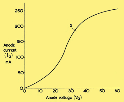
A circuit for obtaining the IaVf characteristic curve of a diode.
Above we have a diode whose filament voltage is controlled by a series variable resistor. A volt-meter connected across the filament tells us the voltage which appears across it. In this instance, we would find it more convenient to employ a diode with a filament rather than one with an indirectly heated cathode because the temperature of the filament will respond quickly to variations in filament voltage. We could obtain exactly the same results if we used a diode with an indirectly heated cathode but we would have to wait for the cathode to settle down to its new temperature after each adjustment of the heater voltage. A current-reading meter in the anode circuit indicates the anode current, and the anode voltage remains constant whilst the curve is being plotted. We will assume that the correct filament rating for the diode is 5 Volts. Such a filament voltage is, in fact, commonly encountered amongst directly heated HT rectifiers (e.g. the 5Y3, which has two diodes and a common filament).
The resultant anode current-filament voltage, or IaVf (with 'f' standing for filament) curve appears below.
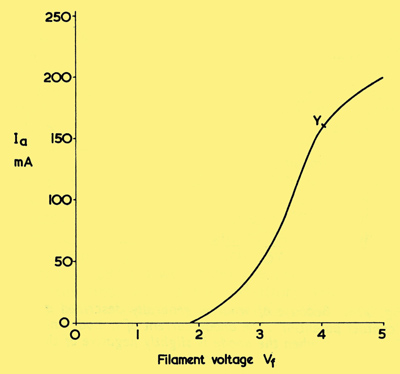
A typical IaVf curve. A fairly low anode voltage, capable of allowing space charge limitation of current to occur after point Y is assumed. The similarity in shape to the IaVa curve may be noted.
For values of Vf below about 2 Volts the filament does not reach emitting temperature, and there is no anode current. At about 2 Volts there is a small amount of emission. All the electrons emitted are attracted towards the positive anode and an anode current commences to flow. As Vf is raised the filament becomes hotter and there is an increased anode current, this still being given by the total emission from the cathode. This process continues until, at about point Y, the filament voltage is such that the filament is approaching its correct running temperature. A relatively high quantity of electrons is now being emitted and a space charge commences to appear, this offering repulsion to further electrons emitted from the cathode. Raising filament voltage still further results in an increasing electron emission, together with a stronger space charge giving greater repulsion to the further electrons emitted by the cathode. Thus, after about point Y, the anode current is limited by the space charge and, since increasing filament voltage does not cause the corresponding increase in anode current which occurred previously, the curve begins to flatten off.
Despite their similarity of shape, the curve of IaVf offers an intriguing contrast with that of IaVa. From the zero point to point Y of the IaVf curve the anode current is limited by saturation, because all electrons emitted by the cathode pass to the anode. After point Y the curve flattens off because of the limitation in current given by space charge. In the IaVa curve, from the zero point to point X, is the result of current limitation by space charge whilst, after point X, the current limitation is due to saturation.
This brief examination of the IaVf curve for a diode is helpful because it enables us to appreciate more fully the limiting of anode current either by space charge or by saturation. The anode voltage which provides the curve above of is sufficiently low to allow a space charge to form when the filament approaches its correct running temperature. To complete the picture we should now draw another graph in which the anode voltage is sufficiently high to give saturation even when the filament reaches its proper operating temperature at a Vf of 5 Volts.
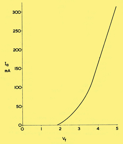
Increasing anode voltage, so as to cause saturation at full filament voltage, changes the Ia Vf curve to that shown here.
The above graph indicates a continually increasing anode current with no flattening off, because the current is at all times limited only by saturation.
Contact Potential
When we discussed the IaVa curve we said that zero anode current flowed at zero anode voltage. This statement is not entirely true, however, and if we examine the IaVa characteristic of a typical diode at low values of anode voltage we will find that the anode current drops to zero only when the anode is made slightly negative of the cathode. At zero anode voltage a small anode current flows, as is illustrated by the curve of below.
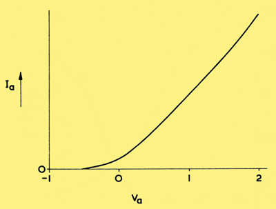
Because of what is generally described as 'contact potential', the anode current of a diode only falls to zero when the anode is slightly negative of the cathode.
This effect can be generally ascribed to 'contact potential'. Contact potential is, basically, the term applied to the small EMF which may be produced when two dissimilar conductors are brought in contact. In a diode the surfaces of the anode and cathode will almost inevitably consist of dissimilar materials, and it can be shown that, when no external EMF is applied to these two electrodes, potentials similar to those which give the contact potential effect appear immediately over their adjacent surfaces. These potentials, in combination, can be looked upon as providing a small internal EMF. in series with the anode voltage, the internal EMF having a polarity such that anode current still flows when the anode voltage is zero. Anode current only falls to zero when the anode voltage is made slightly negative to counteract the contact potential.
In the curve shown above, the contact potential is such that as to permit zero anode current at an anode voltage of about -0.5. However, the actual voltage at which zero current occurs will vary for different diodes and, also, for other factors including the initial electron velocity from the cathode and the amount of gas left in the envelope.
The writer introduced the term 'contact potential' in inverted commas because, although widely accepted as the general term for the effect shown, it defines a phenomenon in which there are other contributory factors. Some textbooks similarly qualify the term when applying it to the overall effect.
Anode AC Resistance
We may now, with the aid of the diode, very conveniently introduce a concept which will be of considerable assistance to us when, later, we come to examine more complex valves.
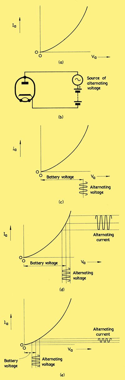
(a) The lower section of a typical IaVa curve for a diode
(b) Connecting a source of alternating voltage, in series with a battery, to the diode
(c) The battery and alternating voltages may have values which cause them to appear along the Va dimension of the graph in the manner shown here
d) Taking lines from the alternating voltage to the curve, and then carrying these to the right, enables the amplitude of the alternating current to be found
(e) Applying the alternating voltage to a lower part of the curve results in a considerably smaller alternating current.
Diagram (a) shows the lower part of the IaVa curve of a diode. We apply to the diode anode a source of alternating voltage in series with a battery, as is shown in (b). Our next step consists of giving values to the battery voltage and the alternating voltage which cause them to be applied to the IaVa graph as shown in (c). What we now want to find is the alternating current which flows in the circuit.
This may be done very readily by drawing lines up to the curve from the centre and peak amplitude levels of the alternating voltage. The points at which these lines meet the IaVa curve will then tell us the corresponding currents, whereupon we may produce lines from these to the right and reconstruct the alternating waveform in terms of current. These processes are carried out in (d), in which the waveform on the right of the graph indicates the alternating current which flows.
In (e) we repeat the process once more, but this time with a lower battery voltage. Once again the waveform representing the alternating current appears on the right but, as is obvious from the diagram, it now has a much lower amplitude. So far as the source of alternating voltage is concerned, the conditions obtaining in (e) are such that, for the same alternating voltage, less alternating current flows than occurred in (d). We may say, therefore, that the situation of (e) corresponds to a greater AC resistance than does that of (d). It is obvious that this AC resistance has increased because the alternating voltage has been applied to a part of the IaVa curve having a different degree of slope.
If, in (d), the RMS value of the alternating voltage were 1 Volt, and the corresponding RMS value of the resultant alternating current were 5 mA, then, from R = E/I the a.c. resistance offered is 200Ω. In (e), the RMS value of the alternating current could be about 2 mA, whereupon the AC resistance in this case becomes increased to 500Ω.
In practice, it is not necessary to draw alternating voltages and currents to find the AC resistance at particular parts of an IaVa curve, and a much simpler method consists of drawing a tangent to the curve at the point selected, as in (a) below, and measuring its slope in terms of voltage and current.
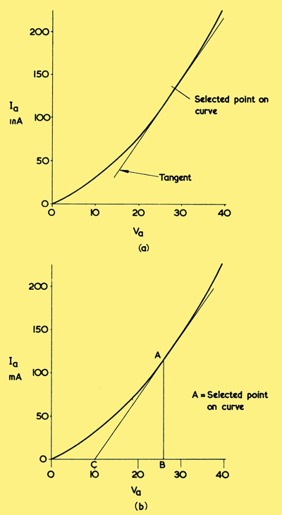
(a) Drawing a tangent to the IaVa curve at the point where it is desired to measure the AC resistance
(b) All that is then required is to measure the slope of the tangent, and one way of doing this consists of producing the tangent to the zero current line. The AC resistance is voltage CB divided by current AB.
Thus, if we continue the tangent to the zero current line and draw a vertical line to the point at which the tangent meets the curve, as shown in (b), dimension AB will show the current which corresponds to the voltage between C and B. In the example shown, the voltage between C and B is 16 and the current (AB) is 115 mA, with the result that the AC resistance at point A is 16/115 x 1,000 = 139Ω.
As was mentioned earlier, we assume, when referring to valve characteristics, that the cathode remains fixed at zero voltage. Our alternating voltage is assumed to be applied, therefore, to the diodes anode, whereupon the AC resistance offered is described as the anode AC resistance, or anode impedance, of the diode. It is most important to note that the anode AC resistance has no connection what so ever with the DC resistance offered by the diode. At point A in (b) a direct voltage of 26 causes a direct current of 115 mA to flow, whereupon the DC resistance becomes 226Ω. The AC resistance is, as we have seen, quite a different figure, and it depends upon the alternating current which flows when an alternating voltage is applied. The abbreviation employed for anode AC resistance is 'ra'.
|