|
In this series of articles the path of the signal through the circuits of the superheterodyne receiver is explained stage by stage.
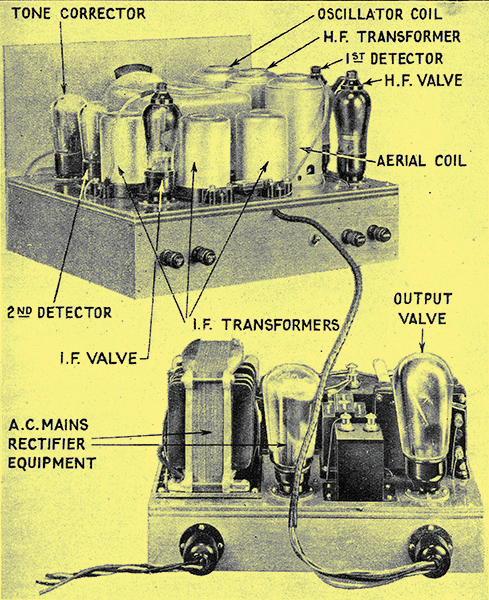
Illustration of a typical superhet, The Wireless World Monodial, with the various parts identified.
The Frequency Changer and IF Amplifier
A new circuit for minimising interference in the superheterodyne receiver.
The course of the signal has now been traced as far as the grid of the first detector and we have briefly dealt with the oscillator. Inspection of the general circuit diagram published with the first part of this series will show that the coil between the points 6 and 2 of the oscillator coil assembly is coupled to the tuned winding and is connected in the cathode lead of the first detector. Since the grid of this valve is joined to the earth line through a tuned circuit, this coil is really in the grid-cathode circuit of the first detector, and, as a result, a voltage due to the oscillator is applied to the first detector grid as well as that caused by the signals.
Sideband Theory
Ignoring interference for the moment, we thus have two different voltages of different frequencies applied to the first detector - one due to the wanted incoming signal, and the other to the oscillator. The valve is adjusted to work as an anode bend rectifier, so that both sets of voltages are rectified. This is the part of the superheterodyne which is really complicated, for it is not always easy to see just what happens, and there is much misapprehension. For a complete understanding of the operation, a complicated mathematical analysis is necessary, but this is quite beyond the scope of the present article.
Some of the chief considerations involved in the design of the frequency changer will be considered later, and for the present it is sufficient to point out that although the input to the first detector consists of only two frequencies, the output contains many more. Due to the rectification process, there will be currents in the anode circuit of the signal frequency, the oscillator frequency, a frequency equal to the sum of the input frequencies, and a frequency equal to the difference of the input frequencies; in addition, there may be harmonics of all these, and there will certainly be the usual direct current consequent upon all rectification. Thus, if the incoming signal has a frequency of 1,000 kHz, and the local oscillator is adjusted to 1,110 kHz, the currents in the anode circuit will have frequencies of 1,000 kHZ, 1,110 kHz, 2,110 kHz, and 110 kHz.
In general, however, the incoming signal will not be a single frequency, for it will be modulated. Modulated carrier can be considered in two different ways; it can be thought of as a simple wave of single frequency, the amplitude of which is varying at the modulation frequency, or it can be considered as a pure continuous wave accompanied by other similar waves spaced on either side of it by an amount equal to the modulation frequency. Thus, a carrier of 1,000 kHz, modulated by a 5,000 Hz note, can be thought of as a wave of 1,000 kHz, the amplitude of which is varying 5,000 times a second, or it can be considered as being a series of pure continuous waves with frequencies of 1,005 kHz, 1,000 kHz, and 995 kHz. These two different viewpoints of modulation are known respectively as the amplitude variation and the sideband theories, and they mean exactly the same thing. The theories have been the subject of much needless controversy; they are really two different ways of describing the same phenomenon, and they are both accurate and mathematically equivalent. We may choose, therefore, whichever is the more convenient for our purpose, and at different stages of the receiver we can change from one to the other at will. In general, the sideband theory is the simpler.
Band-pass IF Coupling
Let us apply it to the present case, therefore, and suppose that instead of an unmodulated signal of 1,000 kHz, We have a signal of that frequency modulated at 5,000 Hz. The signal input to the first detector, therefore, Will consist of a series of frequencies of 1,005, 1,000, and 995 kHz, due to the signal, and a frequency of 1,110 kHz from the oscillator. The output frequencies, therefore, will be 1,110, 1,005, 1,000, 995, 2,115, 2,110, 2,105, 115, 110, and 105 kHz, and 5 kHz, and possibly harmonics of these. Of these frequencies, that of 1,110 kc/ s is the oscillator frequency; theb group 1,005, 1,000, and 995 kc / s is the signal frequency with its sidebands; the group 2,115, 2,110, and 2,105 kHz is a new frequency with sidebands due to the sum of the input frequencies; the group 115, 110, and 105 kHz is another new frequency with sidebands due to the difference of the original frequencies; and the 5 kHz frequency is the normal demodulation of the signal. Of this welter of frequencies in the output, it is the two new groups which interest us the 2,110 kHz and the 110 kHz groups. The first thing to notice is that each group forms the equivalent of a modulated carrier of new frequency, but with the modulation unchanged. Thus, the first group is equivalent to a carrier of 2,110 kHz modulated by a 5,000 Hz note, and the second to a carrier of 110 kHz also modulated at 5,000 Hz. Either of these groups can be treated in exactly the same manner as an incoming signal of the same frequency; it can be amplified and passed through selective circuits until finally it is rectified in order to separate the 5,000 Hz, or other modulation from the carrier in the usual way.
For reasons to be dealt with later, it is the general practice to make use only of the low frequency, the 110 kHz, components of the first detector output, and this is termed the intermediate frequency. A tuned circuit resonating at this frequency, therefore, is included in the anode circuit of the valve in order to select the intermediate frequency and reject all the others. The design of such a circuit follows normal HF amplifier practice, save that it is not usually permissible to connect the first detector anode to a tapping on the coil nor to use a normal type of HF transformer. The matter is not usually so important with a screen-grid first detector valve as with a triode, but it is usually desirable that there should be a capacitor connected between the valve anode and some point at earth potential.
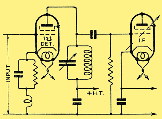
Fig. 1. - A tuned anode IF coupling can be used, but is not usually advisable, since the high-frequency detector output may reach the IF valve grid.
A tuned-anode type of inter-valve coupling would serve admirably, therefore, and the arrangement shown in Fig. 1 would be quite possible. It must not be forgotten, however, that we have a large number of different frequencies in the circuit, of which only the 110 kHz group is required. Even though it maybe very small, the tuned anode circuit offers some impedance at the highest frequency, so that with this simple coupling an appreciable voltage due to the unwanted frequencies may find its way to the grid of the next valve. These frequencies serve no useful purpose at this point, and their presence tends to reduce the input handling capacity of the valve for the wanted signal. It is the general practice, therefore, to use a considerably more selective type of inter-valve coupling, and the circuit of Fig. 2 is commonly employed.

Fig. 2. - A band-pass IF coupling is the most satisfactory, for it gives high selectivity, and largely prevents unwanted frequencies from reaching the IF valve.
Use of Variable-μ Valve
With this arrangement there is no direct connection between the grid of the IF valve and the anode of the first detector, and the coupling is entirely through the mutual inductance between the two coils. Each circuit is tuned to the intermediate frequency, and the coupling between the coils is adjusted to give the desired type of resonance curve. Since the selectivity with two circuits is much greater than with only one, it is found that only the intermediate frequency group of the first detector output can reach the valve grid at any appreciable strength.
In the general receiver circuit an even more complex coupling is employed, and no fewer than four tuned circuits are connected between the first detector and IF valve. The filter is built up from a pair of double-tuned or band-pass circuits similar to those of Fig. 2 coupled together by a small capacitor C11. Through the use of this multiplicity of circuits a very high degree of selectivity is obtainable.
The voltages appearing across the terminals of the last of these four circuits are applied to the grid of another variable-μ valve which acts as the IF amplifier. Its operation is identical with that of the HF valve, save that it works at a different frequency, and it is coupled to the second detector through a pair of tuned circuits which act as a band-pass filter. The valve is biased negatively by the same amount as the HF valve, and its cathode, in fact, is connected directly to that of the HF valve. The variations of bias imposed on the latter for volume control, therefore, occur also on the IF valve, so that the amplifying power of both is reduced simultaneously.
The load impedance of an IF valve is not so important as that of the HF stage, since cross-modulation effects are far less likely to occur. From the point of view of distortion, of course, it is still advisable to keep the load impedance at a moderate value. It is found, however, that the usual type of IF transformer is entirely satisfactory in this respect, for the dynamic resistance of the tuned circuit is about 100,000 Ω.
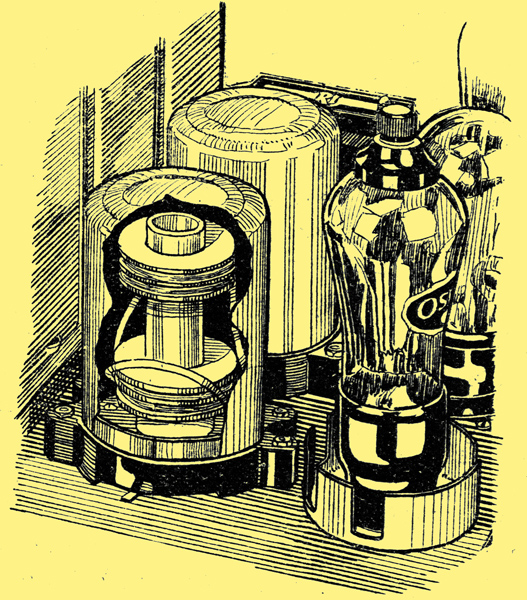
Two typical IF band-pass coils with adjustable coupling are shown in this illustration.
Series Contents
|