|
Designing inter-valve couplings for high frequencies
When the low-frequency currents in television extend from a lower limit than we are accustomed to cater for in sound reproduction well into the radio-frequency spectrum, it is not surprising to find that their amplification involves special technique. This article deals in some detail with the design of suitable amplifiers, and it is shown that it is by no means difficult to obtain an even response over the enormous range of 25 Hz to 1 MHz.
It has been pointed out many times in The Wireless World that high-definition television, of the 25 pictures 240 lines type, demands modulation frequencies up to about 1 MHz. The range of frequencies theoretically required for perfect results is infinite, but in practice a very close approach, to perfection is obtained if all frequencies between some 25 Hz and 1 MHz are properly reproduced. As a result, the low frequency (video) amplifier must be of special design if it is to handle this wide range of frequencies faithfully. The term low frequency is really a misnomer when the frequencies in question extend well into the range which we are accustomed to call high or radio frequencies. It is suggested, therefore, that the term, modulation - frequency is more suitable, since the circuits have to deal with those frequencies by which the carrier is modulated.
Before considering the type of couplings which must be used in the modulation-frequency. amplifier, it is well to review briefly the requirements. The frequency response, as already stated, must be flat within very few decibels over the whole range of frequencies from 25 Hz to 1 MHz. The detector output voltage which operates the amplifier is at present unknown, for we have not yet dealt with this important piece of apparatus, which presents specially difficult problems in television reception. The output is, however, very unlikely to exceed 1 Volt peak. The cathode ray tube requires an input of some 20 Volts RMS or 28 Volts peak. It is essentially a voltage operated device like a valve, so that a power output stage will not be needed in our amplifier. The output valve, therefore, need not necessarily differ from those used in the earlier stage, and the total gain of the amplifier must be at least thirty times.
Valve Input Impedance
Turning now to a consideration of inter-valve couplings, it is obvious that transformers will be unsuitable for the wide frequency range required, and we must turn to resistance coupling. This was dealt with very, fully in recent issues of The Wireless World [★] January 11 & 18, 1935. See extras menu., and as far as pure resistance coupling is concerned the data given there applies fully to television amplifiers. The choice of coupling capacitors and grid leaks for the maintenance of an even response at the very low frequencies must be made entirely on the lines dealt with in that article, and will not be considered here.
It was shown that the response at high modulation frequencies, however, is largely dependent upon the stray circuit capacities, but that with modern triode valves of high mutual conductance and low AC resistance no difficulty is experienced in obtaining an even response up to 10 kHz. This is very far from being the case when the response must be good up to a frequency one hundred times as great!
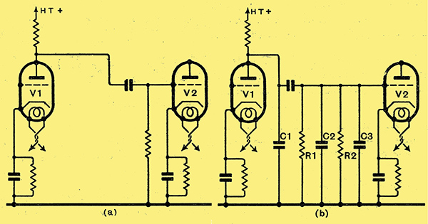
Fig. 1. - The basic connections of a resistance-coupled stage are shown at (a), and the effective circuit at (b), including the stray capacities and the input impedance of V2.
The response obtained from the ordinary resistance-coupled amplifier always falls off at high frequencies, and there are two effects which are responsible for this, one,is caused by the inevitable stray circuit capacities and the other by feedback through the inter-electrode capacity of the valve following the coupling. Although the first effect is by no means unimportant; the second is responsible for most of the loss at high modulation frequencies when triode valves are used. Fig. 1 (a) shows the fundamental circuit of two triodes with resistance-capacity coupling, but the true circuit taking into account the stray capacities is represented by Fig. 1 (b). Here C1 is the anode-cathode capacity of V1 with the addition of the stray wiring capacities, and C2 is the grid-cathode capacity of V2; both these capacities, are constant and are actually real capacitors formed by the proximity of the various electrodes in the valves and their leads.
The capacitor C3, however, is different and has no physical existence as a capacitor. It represents a portion of the input impedance of V2, which is due to feed-back through the anode-grid capacity of this valve. Actually, due to this feed-back, the valve imposes a load upon the coupling and the easiest way of allowing for this is to consider the valve to be perfect and include imaginary components C3 and R2 in the grid circuit which exactly represent the effect of its imperfections.
The values of these components depend not only upon V2 but on the magnitude and nature of its anode circuit load impedance. When this load is a pure resistance at all frequencies, the input resistance R2 is infinite and so need not be considered; the input capacity C3 has a value which is (1+A) times the grid-anode capacity of V2, Where A is the amplification given by V2. In, cases where the anode load is capacitive the input resistance may become very small, and if the load be inductive the resistance may be negative, and so cause instability if tuned couplings be used.
With uncorrected resistance-coupled amplification, the load on V2 consists of a resistance and capacity in parallel, and the exact expressions for the input resistance and capacity become somewhat complex. The amplification of V2 falls with increasing frequency, and in consequence of this C3 is not a constant capacity but one which falls with frequency. In an actual case, with an MHL4 valve, C3 had a value of 100 pF at low and high audio-frequencies, but as the frequency was raised above 10 kHzthe capacity fell until at 1 MHz it was about 60 pF. If this capacity were the only effect, it would not necessarily prohibit the use of triodes, but the input resistance exhibits even greater changes. At frequencies within the audible range, R2 is usually so high that its can be ignored. At 1 MHz, however, it may fall as low as 3 kΩ! There is no way of correcting. for the effects of such an input resistance, as we can for capacity, apart from limiting the gain of the preceding stage by using a load resistance which is small compared with 3 kΩ. Of course, the input, resistance can be kept highs by using a suitably designed load, for V2; but this would almost certainly involve, a tuned circuit for the load, and as such, an arrangement would be necessary for the preceding stage also, there would be grave danger of the input resistance becoming negative and, causing instability. In addition, small changes in the values of components would have a large effect upon the input impedance of the valve.
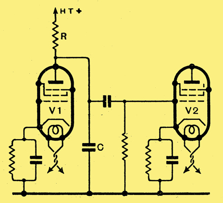
Fig. 2. The input impedance of a screen-grid valve is normally no more than its grid-cathode capacity, so that the resistance-coupled amplifier can be exactly represented by this diagram, where C includes the total shunt capacity.
The screen-grid valve or screened HF pentode represents the solution to the difficulty, for with valves of this type the grid-anode valve capacity is so small that it may be ignored completely, at any rate in a preliminary design. The effective circuit diagram then becomes that of Fig. 1 (b) with both R2 and C3 removed, and this is shown in Fig. 2; in which the capacities of the two valves C1 and C2 have been combined and are represented by the single capacitor C, to which we can assign a value of some 35 pF without much error in most practical cases. With a valve such as the MSP4, a value for R of some 25 kΩ gives the maximum linearity together with a stage gain of about 50 times at low and medium frequencies.
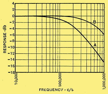
Fig. 3. - The response curves of a single resistance-coupled stage in which the stray capacity C totals 35 pF; (A) is for a coupling resistance R of 25,000 Ω, and (B) for a resistance of 7,900 Ω.
When the capacity C of Fig. 2 has a value of 35 pF, the response at frequencies over 10 kHz is shown by curve A of Fig. 3, and it will be seen that above 100 kHz it falls off very badly indeed. By reducing the value of the coupling resistance the response can be made much more even, as shown by curve B, for a resistance of 7,900 Ω, so that even 1 MHz the loss is only 6 dB. This improvement, however, has been obtained at the expense of amplification, which has fallen to about 15.8 times. In addition, the reduction in the load on the valve restricts the maximum undistorted voltage output of which the valve is capable.
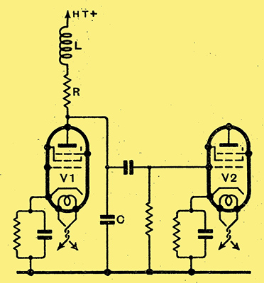
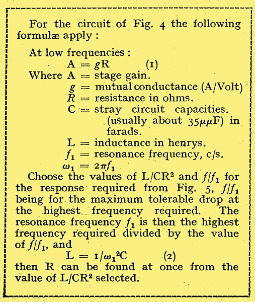
Fig. 4. - By including a coil L in series with the coupling resistance R, a flat response can be secured when the correct values are assigned to the components. (Click image for formulae.)
Now if we insert an inductance L (Fig. 4) in series with the coupling resistance and the correct values be assigned to the various components, it is easy to secure nearly constant amplification. The important factors in design are the frequency at which the circuit resonates and the value of L/CR2, for with screen-grid valves the internal AC resistance is usually so high that it can be neglected, and this also applies to the grid leak of the following valve. The necessary formulae will be given next week and with the aid of these and the curves of Fig. 5 a stage of almost any frequency characteristics can be designed.
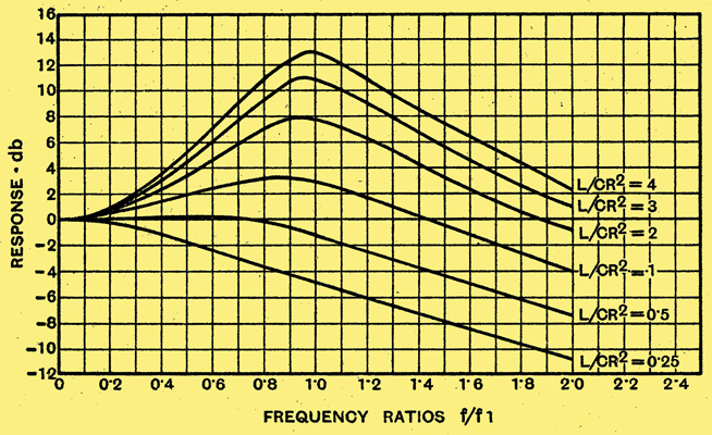
Fig. 5. - The design of corrected amplifiers is facilitated by these curves, which are the frequency response curves of a single stage for various values of L/CR2. Frequency ratios are used to make them of universal application.
As an example of their use, let us consider the design of a stage which shall be as flat as possible with a drop of 3 dB at 1 MHz. From Fig. 5 we can see that the most even response is given by L /CR2 = 0.5, for the curve is nearly flat for values of f/fI up to 0.8. For a loss of 3 dB f/fI = 1.27, so that we find that the resonance frequency is equal to 1,000,000/1.27 = 787,000 Hz; C is fixed by the stray circuit capacities at some 35 pF, so that we are in a position to calculate L and we find it to be 1.75 μH. The value of resistance follows from the chosen value of L/CR2, and in this case is 8,200 Ω. The stage gain at low frequencies is the product of mutual conductance and R, and if the mutual conductance of the valve be 2 mA /V, it is 16.4 times. If desired, the complete response curve can be plotted by substituting the appropriate frequencies for the frequency ratios of Fig. 5, and the response for this case is given by curve A of Fig. 6.
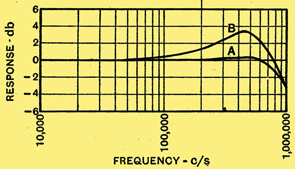
Fig. 6. - The response given by one corrected stage with C = 35 pF. Curve A is for L= 2,530 μH and R = 8,500 Ω, whereas curve B is for L = 1,175 μH and R = 8,200 Ω.
Had a value of I been chosen for L/CR2, the characteristics would have been those of curve B and the stage gain some 17 times.
Designing an Amplifier
The difficulties attendant upon the use of triode valves in the modulation-frequency stages of a television receiver were discussed above and it was shown that these largely disappear if screen-grid valves be used. Even then it is necessary to resort to special corrected couplings, and a series of curves was given which, with the formulae which accompany this article, enable the design to be rapidly carried out, It will be found, however, that although there is no difficulty attached to the attainment of an even response, even at the highest frequencies required in television with a stage gain of a satisfactory, but not high, order, this involves the use of only a moderate load resistance on the valve. Consequently, the maximum undistorted output obtainable is somewhat restricted. This is of little importance in the case of early stages where the output required from the valves is small, but it may be prohibitive in the last stage. This stage feeds the cathode ray tube and should give an output of some 28 Volts peak - for an average high vacuum tube. Now, I if the stage gain is 16 times only, the input to this valve must be 28/16 = 1.75 Volts peak, and the normal operating grid bias for the MSP4 is 1.75 Volts. To be free from any risk of grid current, however, the input cannot exceed about 0.75 Volt peak, so that we cannot safely operate with a lower stage gain than 38.6 times, which means a load resistance of about 20,000 Ω. We shall be wise, therefore, in choosing the optimum value of 25,000 Ω, with which the stage gain is 50 times, for then the input is only 0.56 Volt peak, and there is no danger of grid current.
The response curve of the last stage will then be like curve A of Fig. 3, above, and if we are to obtain a flat overall response from our amplifier the preceding stage must not be flat, but have a rising characteristic. A certain amount of trial and error must enter the design at this point. The loss at 1 MHz is 14.9 dB, so that we must choose a characteristic for the preceding stage which rises by about this amount. Fig. 5 shows that when L/CR2 = 4 the rise is 13.0 dB at f/f1 = 1. This response curve replotted on a frequency basis for a resonance frequency of 1 MHz is shown by curve B of Fig. 7, in which curve A is for the last stage. The combination of the two curves gives the results shown at C, with a total gain for the two stages of 220 times. Even now, however, the response is not very good, for although the loss at 1 MHz is only 1.8 dB, there is a drop to 4.2 dB at 450 kHz.
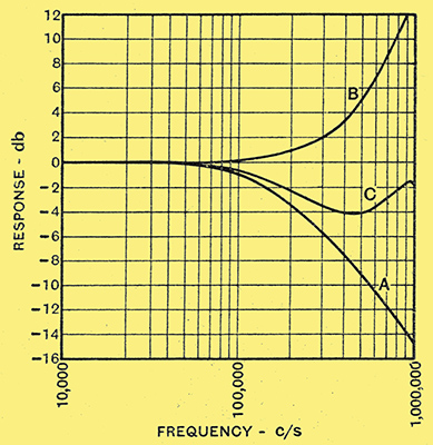
Fig. 7. - Curve A shows the response of the uncorrected output stage, and B that of an over-corrected penultimate stage, while curve C represents their combination.
Now, We cannot readily avoid this type of characteristic when using only a single correcting stage preceding the output valve, for the shapes of the response curves of the different stages are not complementary. We cannot properly correct the output stage, for the load resistance must be maintained at a fairly high value. We can, however, apply a small measure of correction. Suppose we try L/CR2 = 0.5, which gives the flattest response (Fig. 5). Knowing R2 we can calculate L /C, and, as C is known, we obtain the value of L. We can then find the resonance frequency for which f/f1 = 1, and it is 262 kHz. The response curve is then A of Figs. 8, 9, and 10. Curve B of Fig. 8 is for the same preceding stage as before, and curve C gives the new combination; a definite improvement is evident, but it is still not as good as we should like.
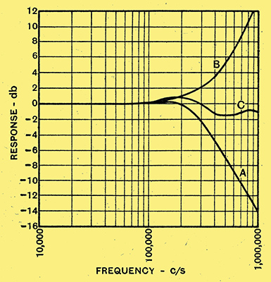
Fig. 8. - Curve A is for a corrected output stage with R = 25,000 Ω and L = 10,900 μH., while B and C are respectively the penultimate stage and the overall with L = 725 μH. and R = 2,200 Ω.
The Corrector Stage
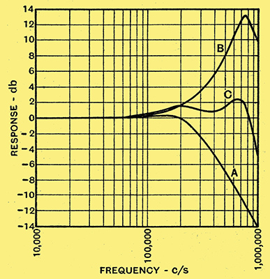
Fig. 9. - Curve A is the same as in Fig. 8, but, in curve B, L = 1286 μH. and R = 3,000 Ω. This gives the overall response of curve C.
It is usually better to have a greater drop at the highest frequency and a more even response at lower frequencies. Let us try, therefore, peaking the first stage at 750 kHz instead of 1 MHz the response of the first stage is given by curve B of Fig. 9 and the overall response by curve C. The total gain has now risen to 300 times, but the characteristic is still not very satisfactory, for the loss at 1 MHz is some 5 dB, and there is a rise of 2.2 dB at 650 kHz. It is evident that the corrector circuit is now resonating at too low a frequency, so let us try 850 kHz.
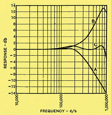
Fig. 10 - Curve A is again the same as in the preceding illustration, but curve B is now for values of L = 1,000 μH. and R = 2,670 Ω, and curve C represents the overall characteristics.
The results are shown in Fig. 10. in which, as before, curve B represents the first stage and curve C the overall characteristic. It is evident that we have now found a combination which is likely to meet even exacting requirements. The response is even up to 50,000 Hz, after which it rises gradually to a maximum of +1.2 dB at 175,000 Hz; it then falls to a minimum of -0.2 dB at 450,000 Hz, after which it again rises to +1 dB at 800,000 Hz. The fall at higher frequencies is rapid, but at 1,000,000 Hz it is only -2.9 dB, so that it is clear that this combination is likely to be highly satisfactory.
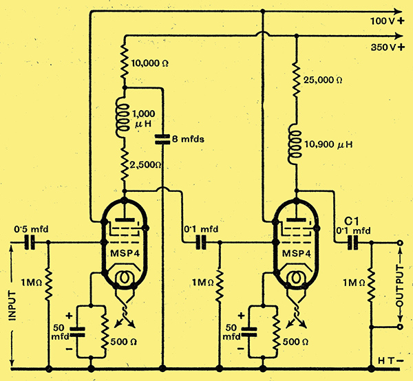
Fig. 11. - The circuit diagram of an experimental amplifier. With the values of components. shown, the frequency characteristic is that of Fig. 13.
In order to check the design an amplifier was built embodying components of the values which have just been calculated and its circuit diagram appears in Fig. 11. No doubt was felt on the validity of the design calculations, but it was known that these contained certain approximations; in particular the self-capacity of the correcting coils has been ignored, and it would not be quite accurate to treat it merely as increasing the general circuit capacity owing to the presence of the coupling resistance. Moreover, in any practical amplifier unsuspected effects are likely to be found, and feedback through stray couplings might appreciably modify the characteristics.
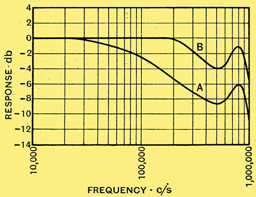
Fig. 12. - These curves represent the initial response with the amplifier of Fig. 11, and the high-frequency attenuation is due to excessive stray capacity in the output circuit. The substitution of a Bakelite for a metal-cased capacitor, C1, altered the response from curve A to curve B.
When first tried out the amplifier of Fig. 11. gave the measured response curve A of Fig. 12 for frequencies above 10,000 Hz with a gain of 196 times, and this is obviously very different from the calculated,curve C of Fig. 10. The discrepancy was far too great to be ignored, and in order to find out where the trouble lay the characteristics of the output stage alone were measured and found to exhibit a similar departure from the expected values. The reason was discovered to lie in the fact that the stray capacity across the output circuit was 64 pF instead of the value of 35 pF assumed in the calculations.
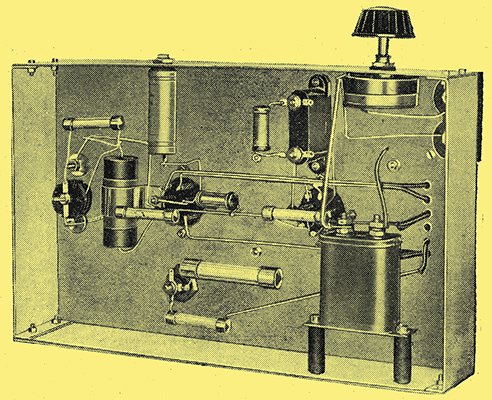
An under base view of the experimental amplifier. Note the insulating mounting of the metal-cased fixed capacitor to avoid the effect described in the text.
The input capacity of the valve voltmeter employed for measuring the output voltage was known to be 15 pF, but this was intended to be included in the 35 pF for the total capacity, since in normal operation the cathode-ray tube will have about this capacity with its associated wiring. A search for the cause of the high stray capacity, therefore, was confined to the amplifier, and two points were brought to light which well illustrate the need for care in the construction of television amplifiers. The component used for the output coupling capacitor C1 (Fig. 11) was of the metal-case type, and measurement showed it to have a capacity of 23 pF between its terminals and the case. The metal case was earthed by its contact with the chassis, so that this 23 pF was fully effective in augmenting the stray capacity. On changing this capacitor for one of the Bakelite-case type the response curve B of Fig. 12 was obtained, and a comparison with curve A well illustrates the need for care in the choice of components.
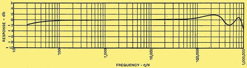
Fig. 13. - The final response of the amplifier is shown here, and it is fiat within ± 2 dB from 20 Hz to 900,000 Hz.
The stray capacity was still high however, being now 41 pF, and the cause of this was found to lie in the arrangements made for the output connections. A multi-way terminal-connector was used and the high potential output terminal was sandwiched between two at earth potential. Omitting the terminal entirely and using in its place the capacitor terminal on C1 itself reduced the capacity to a figure slightly below 35 pF. The complete response curve then took the form shown in Fig. 13, and although it still exhibited some variation from the calculated response, this was not considered serious enough to warrant further investigation.
This curve is very satisfactory indeed, for the amplifier employed is in no way complicated, and the only components used which would not be needed in a similar amplifier for sound purposes are the two correcting chokes, which should not cost more than a few shillings. At the low frequency end the response commences to tall at about 100 Hz, but it does not drop below 1.8 dB even at 20 Hs. This is particularly interesting in view of the fact that it has been stated that cathode biasing cannot be used with HFpentode valves it a good low-frequency response be required. The curve of Fig. 13 shows that there is no difficulty in maintaining the low frequencies if 50 μF electrolytic capacitors be used to bypass the bias resistances.
At higher frequencies the curve is level up to 50,000 Hz, beyond which it rises gradually and reaches a maximum of +1.8 dB for frequencies of 200,000 Hz to 250,000 Hz. The response then falls to a minimum of -1.8 dB at 500,000 Hz, after which it again rises to +0.8 dB at 800,000 Hz. For frequencies higher than this the output steadily falls, and at 1,000,000 Hz the loss is -3.6 dB. The characteristic is actually better than it appears at a cursory glance, for one is at first apt to pay too much attention to the variations at high frequencies. The response is even within ±1.8 dB (a maximum variation of 3.6 dB) over the enormous range of 20 Hz to 940,000 Hz. A variation of this order over the range of 50 Hz to 10,000 Hz is often considered good in a sound amplifier, but the ratio of maximum to minimum frequencies is only 200:1 compared with the ratio of 47,000:1 for the television amplifier!
Before concluding, it may be as well to summarise the chief points which arise in the design of television amplifiers:-
- Triodes cannot be used easily on account of their low input impedance at high frequencies.
- Even with screen-gridB; or HF pentode valves, simple corrector circuits are necessary.
- The most even response is obtained by correcting each stage individually.
- When the output valve must be operated with a high load impedance to avoid amplitude distortion, full correction in this stage is impossible, and the overall response must be maintained by over-correcting a preceding stage. The response is not then as flat as in (3), but can usually be made very good.
- At low frequencies. the design follows normal practice, and no special precautions are necessary. Cathode biasing can be used.
- Care must be exercised in the choice of layout and components in order to keep stray capacities at a minimum.
No mention has been made of phase distortion in this article, in spite of the fact that this may prove important in television reception. It is likely to occur at both low and high frequencies, and the correction circuits employed for maintaining an even response also tend to correct for phase distortion at high frequencies. In general, however, the degrees of correction necessary for a minimum of both types of distortion are not the same. At the present time phase distortion seems less important than the maintenance of an even frequency response, but there is no doubt that it will have to be considered in the future, and the writer hopes to deal with some of its simpler aspects in a further article.
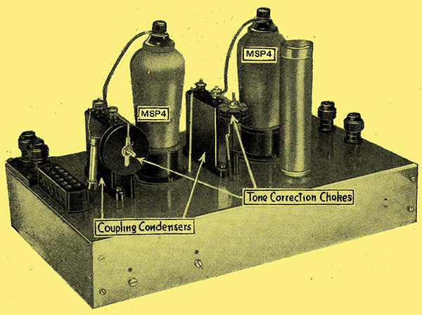
An experimental amplifier designed in accordance with the considerations discussed in this article.
|